Criticality: The Physical and Numerical Models

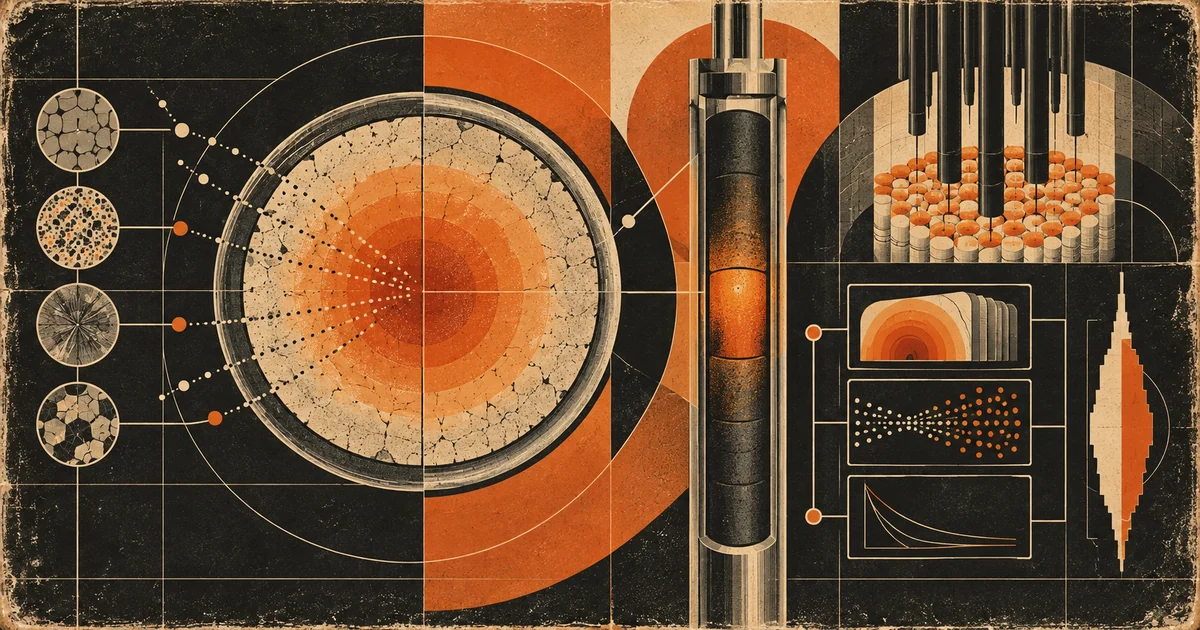
I am a nuclear engineer, and for years I taught reactor behaviour with static diagrams. The medium was the limitation, not the audience. Criticality is a pressurised water reactor that runs in a browser tab. This article describes what is inside it: the physics it solves, the numerical method chosen for each part, how those parts are coupled, what the model is for, and where it stops.

Why a whiteboard cannot teach a reactor

A reactor is at least six systems on six different time constants, all coupled, all moving at once. The prompt neutron population responds in tens of microseconds. Delayed neutron precursors respond over seconds to a minute. The fuel pellet's thermal step response is about four seconds. The primary loop takes ten seconds to go round once. Xenon-135 takes about forty hours to reach equilibrium, and after a shutdown it goes on building for hours more before it peaks. Decay heat has structure from one second out to years.

Every one of those talks to the others. Fuel temperature feeds Doppler feedback, which feeds the neutron population, which feeds fuel temperature; coolant temperature does the same on a slower loop, and xenon closes the same circuit again over hours.

A student can solve each of those equations separately, pass the exam, and still have no idea what the plant does when you pull a rod bank. That is not a failure of the student, it is a failure of the instrument. What needs teaching is a trajectory in a coupled system, and a whiteboard is a static medium. You can draw the xenon curve. You cannot draw the moment when a boron dilution ordered forty minutes ago arrives at the core while xenon is still building in, and the rods have to answer for both.

Training has the same gap from the other side: a new engineer meets procedures before intuition. And most existing teaching tools are instrument replicas, all gauges and setpoints and valve handles. They render the control room, not the phenomenon. So the goal was narrow: show the physics, not the instruments.

The physical models

The engine solves a coupled system of ordinary differential equations for a generic four-loop Westinghouse-class PWR at 3400 MW thermal, plus two boundary value problems that are re-solved rather than integrated.

Point kinetics and the delayed neutron groups

$$\begin{aligned} \frac{dn}{dt} &= \frac{\rho - \beta}{\Lambda}\,n \;+\; \sum_{i=1}^{6} \lambda_i C_i \;+\; S \\[4pt] \frac{dC_i}{dt} &= \frac{\beta_i}{\Lambda}\,n \;-\; \lambda_i C_i, \qquad i = 1 \dots 6 \end{aligned}$$

Six delayed groups, with Keepin's data for thermal fission of uranium-235. That structure is the reason reactors can be operated by human beings. If every neutron were prompt, a small reactivity would multiply the population on a twenty-microsecond clock and nothing built out of moving metal could follow it. Instead a fraction of a per cent of neutrons arrive delayed, from precursors with half-lives from a fraction of a second to nearly a minute, and while $\rho$ stays below $\beta$ the population cannot run away faster than those precursors decay. The reactor's response time is set not by the neutrons but by the isotopes that emit them a minute later.

The prompt jump and the 1/M plot an operator draws during an approach to critical both fall out of these equations rather than being bolted on top of them.

The reactivity balance

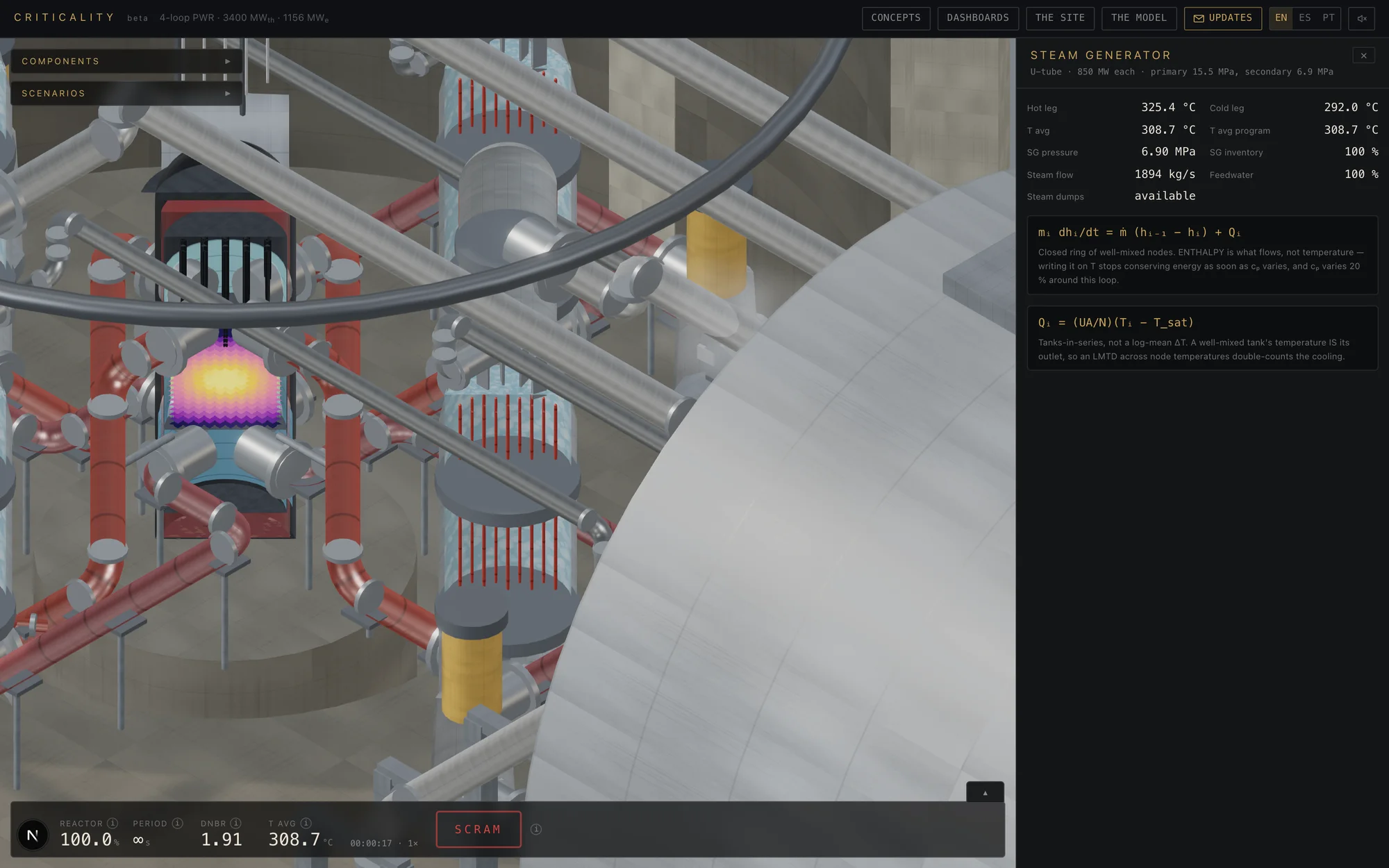
Reactivity is a sum of independently evaluated terms, rods, boron, Doppler, moderator, xenon and samarium, each kept separately in the state rather than accumulated, because the decomposition is the object worth watching.

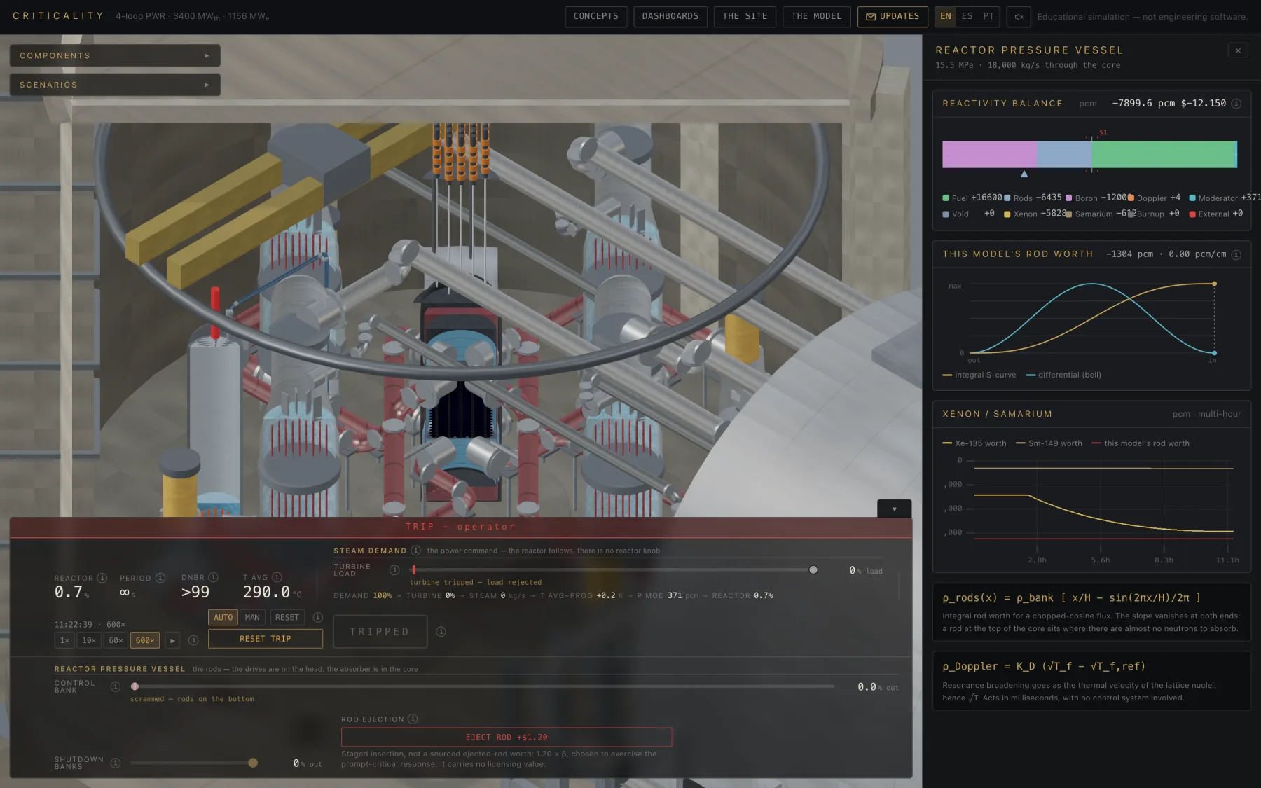
Two of those terms carry most of the teaching. Boron is not an input but a state, driven toward the operator's demand through a lag of tens of minutes, so you ask for boron and it arrives over hours, which forces the operator to plan. Doppler acts on the pellet's conduction timescale with no control system in the loop, which is why it, and only it, can terminate a fast excursion.

The axial flux shape

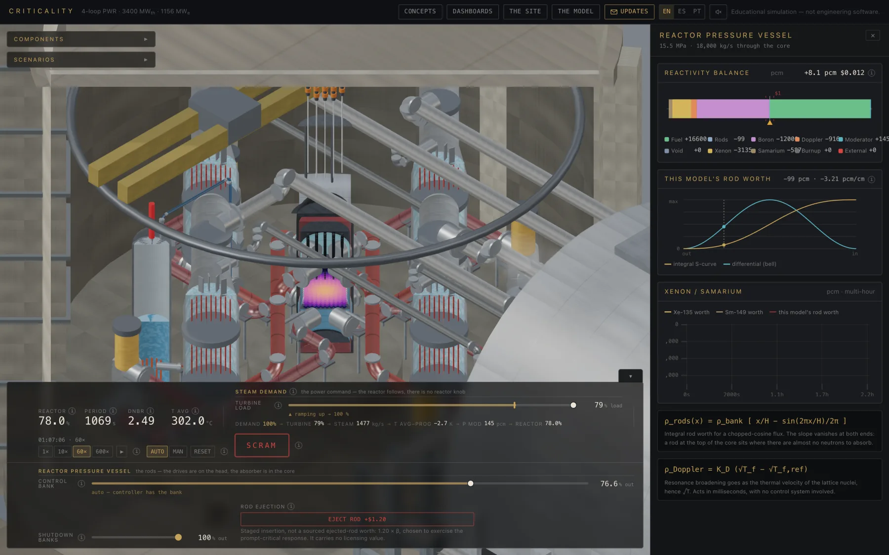
Point kinetics is zero-dimensional: it knows how many neutrons there are, not where. The distribution comes from a separate one-group, one-dimensional diffusion eigenproblem over twenty axial nodes,

$$-D\,\frac{d^{2}\phi}{dz^{2}} \;+\; \Sigma_a(z)\,\phi \;=\; \frac{1}{k}\,\nu\Sigma_f\,\phi$$

with vacuum boundaries beyond the active fuel. A flux shape is the answer to a competition: neutrons are produced where fuel is, absorbed where absorber is, and leak out of the ends, and the eigenproblem finds the one distribution that reproduces itself under it. The core is loosely coupled along its axis, which is why a partially inserted bank produces a genuine local depression rather than a gentle tilt.

The iodine-xenon chain and the shutdown pit

$$\begin{aligned} \frac{dI}{dt} &= \gamma_I \Sigma_f \phi \;-\; \lambda_I I \\[4pt] \frac{dX}{dt} &= \gamma_X \Sigma_f \phi \;+\; \lambda_I I \;-\; \lambda_X X \;-\; \sigma_a X \phi \end{aligned}$$

Iodine-135 has a 6.57 h half-life; xenon-135 has 9.14 h and an absorption cross section of 2.65 million barns, which is why a few atoms per million matter at all.

The whole of the xenon pit lives in that last term. In operation, capture destroys xenon as fast as iodine makes it. Scram, and the flux vanishes: production from iodine decay continues, destruction stops entirely, and the inventory climbs past its operating value for hours before decaying away. A restart a few hours after a trip cannot be bought back with rods, it needs boron the operator has not had time to dilute. A day and a half later it is easy. One detail decides whether any of that appears: the poisons are driven by fission power alone, not total thermal power. Feed total power in and a scrammed core keeps burning xenon out, and the pit disappears.

Radial conduction in the fuel pellet

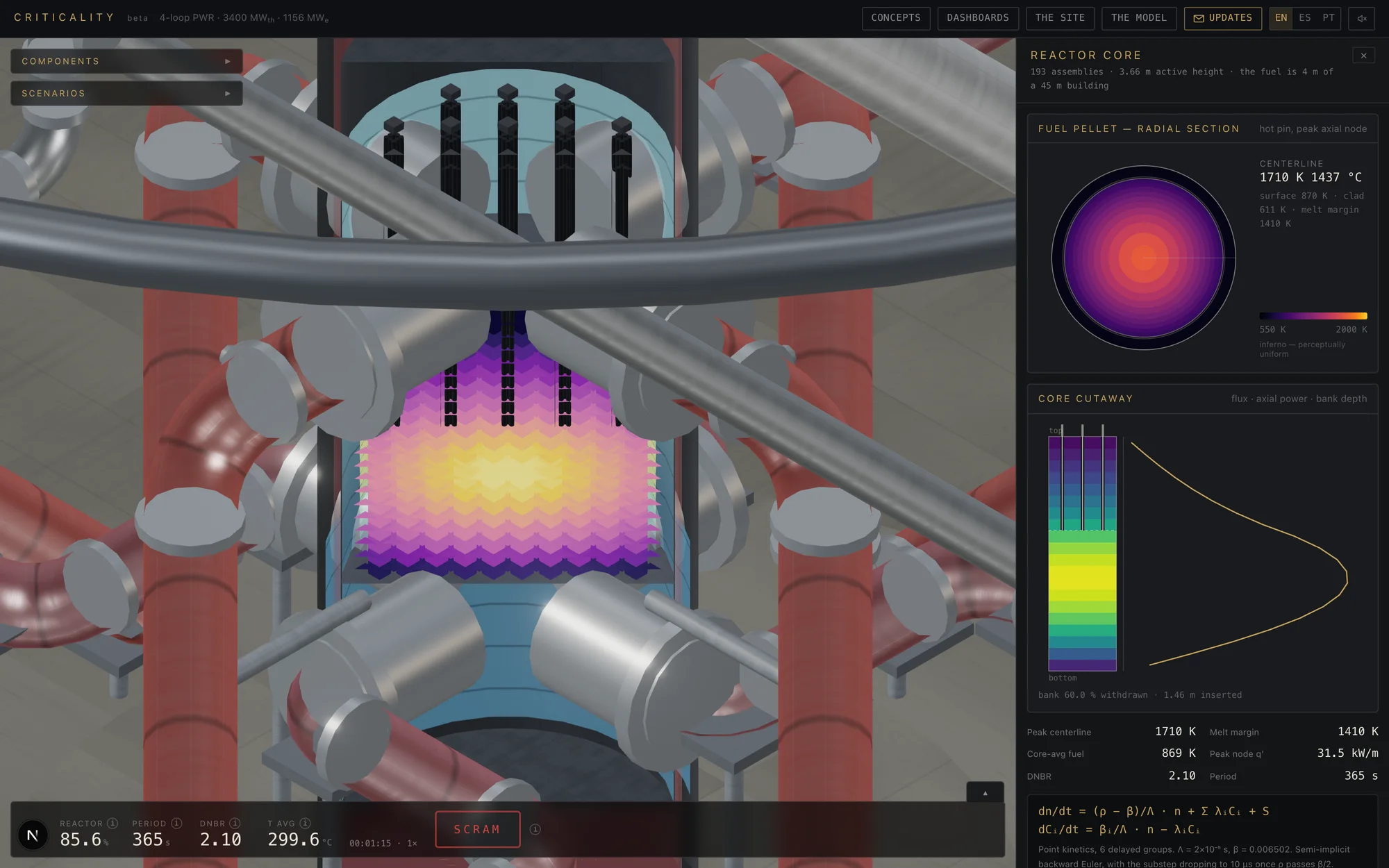
Each axial node carries a one-dimensional radial conduction solve through pellet, gap and cladding:

$$\rho\,c_p\,\frac{\partial T}{\partial t} \;=\; \frac{1}{r}\,\frac{\partial}{\partial r}\!\left( k(T)\,r\,\frac{\partial T}{\partial r} \right) \;+\; q'''$$

The pellet is divided into ten annuli of equal area, so each carries equal volume, equal heat capacity and, the source being uniform, equal power. Two clad nodes follow, and the gap is a resistance at the interface rather than a node. That mesh answers the question students actually ask. Why is the centreline of a pellet hundreds of degrees hotter than its surface, across four millimetres of ceramic? Because uranium dioxide conductivity falls as it heats, by roughly a factor of three over the range a pellet works in, so the hot interior conducts worse than the cool exterior and the profile steepens itself.

The primary loop as enthalpy transport

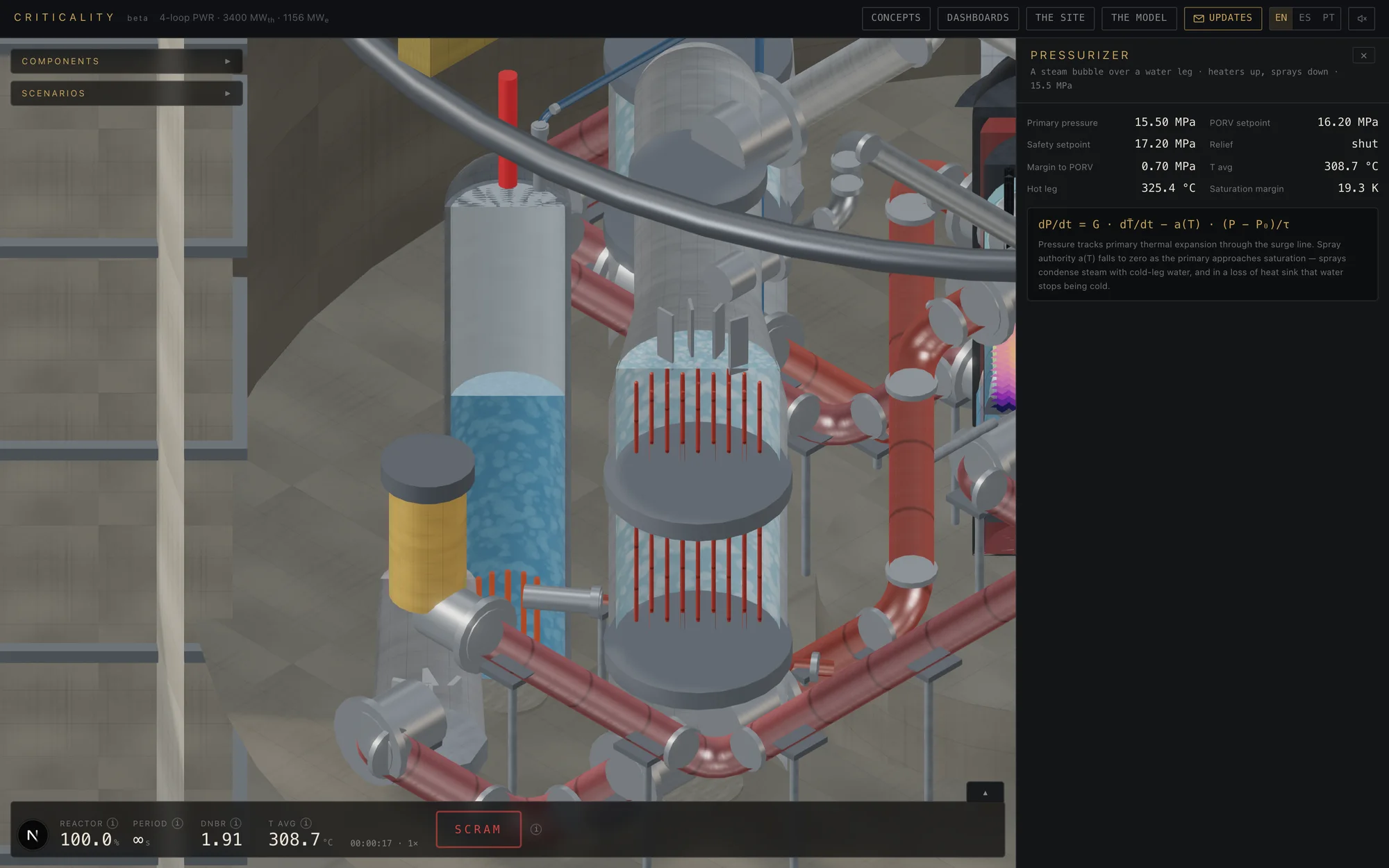
The primary is a closed ring of well-mixed nodes: core, hot legs, steam generators, cold legs. Two nodes per leg approximate plug flow by tanks in series, so the lag between a power change and the hot-leg response shows up on the trends.

The balance is written on enthalpy, not temperature, so the convective terms telescope exactly around the ring and total energy change is core heat minus steam generator heat by construction. The heat driving it is the clad-to-coolant heat returned by the pin solve rather than the fission power, which puts the fuel's thermal inertia in the picture: over the first minute of a scram the fuel gives heat back to the coolant that a generation-based source term would discard.

Decay heat

Nine exponentially decaying fission-product groups, driven by the fission rate exactly as the delayed neutron precursors are, with decay constants spread one per decade. What this makes visible is that a core makes roughly 7 % of rated power the instant it trips, and still needs cooling days later. Because the groups follow the actual power history, the trajectory can be a load follow or a scram from part load without needing a well-defined shutdown instant, and it cannot be zeroed by clearing a trip latch.

The numerical methods

The system spans about eleven orders of magnitude in timescale, from the prompt neutron mode to the slowest decay group. No single explicit step size is both stable and usable, so each subsystem gets the method its own stiffness demands. The choice of integrator here is a physics decision, not a coding preference.

Kinetics: semi-implicit backward Euler, inverted analytically. Writing the precursor update implicitly and substituting into the neutron equation eliminates the precursors and leaves a scalar update: one pass over six groups per substep, no matrix factorisation, which is what makes a microsecond substep affordable in a browser. Backward Euler was chosen over anything explicit or trapezoidal for one reason. It is L-stable: the prompt mode is damped monotonically at any step size, so the integrator lands on the correct quasi-static balance instead of ringing about it. That is what makes fast time acceleration safe.

The pellet: implicit tridiagonal on equal-area annuli. The implicit scheme is forced by the mesh: equal area means unequal width, and the thin outer annuli and clad nodes would cap an explicit step at a few milliseconds. Backward Euler on the finite-volume discretisation gives a tridiagonal system solved by the Thomas algorithm, and the step returns the clad-to-coolant heat at the end-of-step clad temperature, because that is what closes the energy balance at the fuel-coolant interface.

Poisons and decay heat: exact exponential integration. Both chains are linear at fixed flux. Substituting the parent's exponential into the daughter's source puts every equation in the form

$$\frac{dy}{dt} \;=\; p_0 \;+\; p_1 e^{-\mu t} \;-\; a\,y$$

which has a closed-form solution over the step. No truncation error inside the step and no stability limit at all, so nothing in the poison chain ever forces the step to shrink, where a generic Runge-Kutta would spend a forty-hour xenon scenario taking steps sized by the fastest removal rate in the chain.

The loop: classical explicit RK4, because here implicit would be wasted. The fastest loop time constant is orders of magnitude slower than the prompt mode, so the steps in use are far inside the stability limit.

The axial shape: power iteration, memoised. The shape is a pure function of the two bank positions, so it is re-solved only when a bank has actually moved. Sub-stepping, in short, is needed in exactly one place, the neutron kinetics, and nowhere else.

How the models are coupled

One pass over the modules is one coupling block, in a fixed order: the balance produces one scalar, the kinetics turns it into a neutron population, decay heat is added to give core thermal power, the axial solver distributes that power over its nodes, the pin solve produces the temperature field and the clad-to-coolant heat, the loop turns that heat into coolant temperatures, and the poisons close back onto the balance.

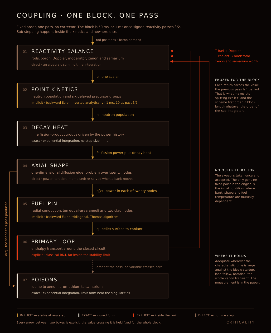
Two of those returns are feedback in the control-theoretic sense, and they are why the ordering matters at all: fuel temperature into Doppler, and coolant temperature into the moderator term.

The scheme is explicit operator splitting with sub-cycling, fast physics inside slow, with everything crossing a subsystem boundary frozen for one block. The block shortens automatically as reactivity climbs toward prompt, so Doppler is not held stale while power runs away. There is no corrector pass and no outer iteration anywhere in the transient: the sweep is taken once and accepted, which makes the scheme first order in block length whatever the order of its sub-integrators, and leaves that one-block staleness as the whole of the residual error.

Explicit splitting is adequate wherever the characteristic time is large against the block, which covers startup, load follow, boration and the whole of a xenon transient. It stops being adequate when the two approach each other, which for this model means a uniform prompt reactivity pulse, and the fix there is a semi-implicit treatment that lets Doppler respond within the block.

What the model is for

It is built to teach reactor behaviour, and to be watched rather than read. For a university course it replaces the static diagram with the thing the diagram was standing in for: run the pellet up in power and watch the profile steepen, insert a bank and watch the flux deform, scram a core that has been at power for forty hours and then try to restart it. For utility and vendor training it fills the gap before the full-scope simulator, where a new engineer needs intuition about why the plant answers the way it does, and where a licensed replica is too scarce and too procedural to be the first tool anyone touches. For outreach it is a nuclear plant anybody can open in a tab.

And for an operator, a vendor or a research group, this generic four-loop PWR is a base to specialise. Every model in it is stated and every constant is either sourced or declared as calibrated, so swapping in a specific plant's rod worths, coefficients and loop geometry is data work on a documented engine rather than archaeology on somebody's black box.

The simulator is in beta and the physics is still being extended. What is described above is what it solves today.

Known limitations

Each of these is a scope boundary rather than a loose end, and each describes what a model delivered for a specific plant would carry instead.

The pellet-clad gap conductance is a single constant, the beginning-of-life value, at every power and every point in the fuel's life. Gap conductance is not a material property; it is the outcome of a thermal-mechanical problem the pellet and the clad solve jointly, and reproducing it is what a fuel performance code is for, whether FRAPCON, TRANSURANUS or BISON, with a materials database and a burnup history this engine does not carry. So the pellet view is a correct picture of conduction under a stated gap resistance, and it is not a statement about fuel integrity.

DNBR here is a margin indicator, not a prediction of plant margin, and the app says so where it is shown. Departure from nucleate boiling is a property of a geometry under a flow, not of a fluid state: a qualified correlation carries the rod bundle it was measured in, which means a subchannel code and an approved bundle correlation. It reads as a trend here, and it is on no other physics path in the engine.

The core has no burnable absorber, and no burnup. A real beginning-of-cycle core holds much of its excess reactivity in gadolinia or IFBA built into the fuel; this one holds all of it in soluble boron, because an absorber that burns out is a state variable rather than an added term.

The primary is single phase. No boiling in the core, no two-phase flow, no loss of coolant, and pump flow steps between settled counts rather than coasting down. This is a model of a plant operating, not of a plant in an accident, and it is deliberately not a safety analysis tool.

The neutronics is point kinetics with a separate axial shape, not spatial kinetics. It reproduces axial redistribution as a bank moves, and it does not reproduce radial or azimuthal tilts, or a local excursion in one region of a core.

I would rather publish that list than a claim I cannot source.

Benchmarks, and a paper

Everything above is a statement about physics, and statements about physics are worth what their evidence is worth. The engine carries a benchmark suite: analytic limits it must reproduce, published reference solutions for coupled kinetics with feedback, and comparisons against measured data from operating plants and from the experimental literature, each with an acceptance band fixed before the run rather than after it.

That work is being prepared as a paper rather than as a blog post, because it deserves a format that lets a reviewer check it. It is coming shortly, and it will be linked here when it is out.

Running the simulator

The simulator is at criticality.fedecaccia.com, with no installation and no account. The most direct demonstration of the coupling described above is to withdraw the control bank while watching the reactivity balance, and then to run at full power for forty hours, scram, and attempt a restart four hours later.

Further articles treat single subjects in more depth, including the xenon transient, the fuel pellet, and the requirements for determinism in a coupled plant model.